import numpy as np
import matplotlib.pyplot as plt
import pandas as pd
from statsmodels.graphics.tsaplots import acf as acf_func

plt.style.use("ggplot")
import arch
import yfinance as yf
import datetime as dt
from statsmodels.tsa.arima.model import ARIMA
We need to model volatility for risk management and trading.
ARCH and GARCH
Conditional Heteroskedasticity is the academic term for volatility clustering. \(\text{ARCH}(1)\) formulation is
\[ \epsilon_t= \sigma_t w_t \] where \(\{w_t\}\) is a white noise process.
\[ \sigma_t^2=\alpha_0 + \alpha_1 \epsilon_{t-1}^2 \] \(\{\epsilon_t\}\) is autoregressive conditional heteroskedastic process with order unity.
A slight modification will show that how \(\text{ARCH}\) models volatility \[\begin{aligned} \operatorname{Var}\left(\epsilon_t\right) & =\mathrm{E}\left[\epsilon_t^2\right]-\left(\mathrm{E}\left[\epsilon_t\right]\right)^2 \\ & =\mathrm{E}\left[\epsilon_t^2\right] \\ & =\mathrm{E}\left[w_t^2\right] \mathrm{E}\left[\alpha_0+\alpha_1 \epsilon_{t-1}^2\right] \\ & =\mathrm{E}\left[\alpha_0+\alpha_1 \epsilon_{t-1}^2\right] \\ & =\alpha_0+\alpha_1 \operatorname{Var}\left(\epsilon_{t-1}\right) \end{aligned}\]Simply put \[ \operatorname{Var}=\alpha_0+\alpha_1 \operatorname{Var}\left(\epsilon_{t-1}\right) \] which is also an \(\text{AR}(1)\).
For \(\text{AR}(p)\) \[ \epsilon_t=w_t \sqrt{\alpha_0+\sum_{i=1}^p \alpha_p \epsilon_{t-i}^2} \]
The counterpart of \(\text{ARMA}\) is Generalised Autoregressive Conditional Heteroskedastic (\(\text{GARCH}\)), usually formulated as \[ \begin{align} \epsilon_t&= \sigma_t w_t\\ \sigma_t^2&=\alpha_0+\sum_{i=1}^q \alpha_i \epsilon_{t-i}^2+\sum_{j=1}^p \beta_j \sigma_{t-j}^2 \end{align} \] We say \(\{\epsilon_t\}\) is a \(\text{GARCH}(p, q)\) process.
GARCH(1, 1) Simulation
\[\begin{aligned} \epsilon_t & =\sigma_t w_t \\ \sigma_t^2 & =\alpha_0+\alpha_1 \epsilon_{t-1}^2+\beta_1 \sigma_{t-1}^2 \end{aligned}\]If \(\alpha_1+\beta_1<1\), the system is stable, otherwise unstable.
Generate \(\text{GARCH}(1, 1)\) data.
def gen_garch11(a0, a1, b1, N):
    w = np.random.randn(N)
    epsilon = np.zeros(N)
    sigma_sq = np.zeros(N)

    for i in range(1, N):
        sigma_sq[i] = a0 + a1 * epsilon[i - 1] ** 2 + b1 * sigma_sq[i - 1]
        epsilon[i] = w[i] * np.sqrt(sigma_sq[i])
    return epsilon
epsilon = gen_garch11(a0=0.2, a1=0.3, b1=0.4, N=1000)Plot generated data and ACFs.
epsilon_acf = acf_func(epsilon, nlags=50)
epsilon_acf_sq = acf_func(epsilon**2, nlags=50)
fig, ax = plt.subplots(figsize=(12, 12), nrows=3, ncols=1)
ax[0].plot(epsilon, label="$\epsilon$")
ax[1].bar(np.arange(len(epsilon_acf)), epsilon_acf, label="$\epsilon$ ACF")
ax[1].axhline(np.std(epsilon_acf[1:]) * 1.96, ls="--", color="b")
ax[1].axhline(-np.std(epsilon_acf[1:]) * 1.96, ls="--", color="b")
ax[2].bar(np.arange(len(epsilon_acf)), epsilon_acf_sq, label="$\epsilon^2$ ACF")
ax[2].axhline(np.std(epsilon_acf_sq[1:]) * 1.96, ls="--", color="b")
ax[2].axhline(-np.std(epsilon_acf_sq[1:]) * 1.96, ls="--", color="b")
for i in range(3):
ax[i].legend()
plt.show()<>:2: SyntaxWarning:
invalid escape sequence '\e'
<>:4: SyntaxWarning:
invalid escape sequence '\e'
<>:8: SyntaxWarning:
invalid escape sequence '\e'
<>:2: SyntaxWarning:
invalid escape sequence '\e'
<>:4: SyntaxWarning:
invalid escape sequence '\e'
<>:8: SyntaxWarning:
invalid escape sequence '\e'
/tmp/ipykernel_4645/683653153.py:2: SyntaxWarning:
invalid escape sequence '\e'
/tmp/ipykernel_4645/683653153.py:4: SyntaxWarning:
invalid escape sequence '\e'
/tmp/ipykernel_4645/683653153.py:8: SyntaxWarning:
invalid escape sequence '\e'
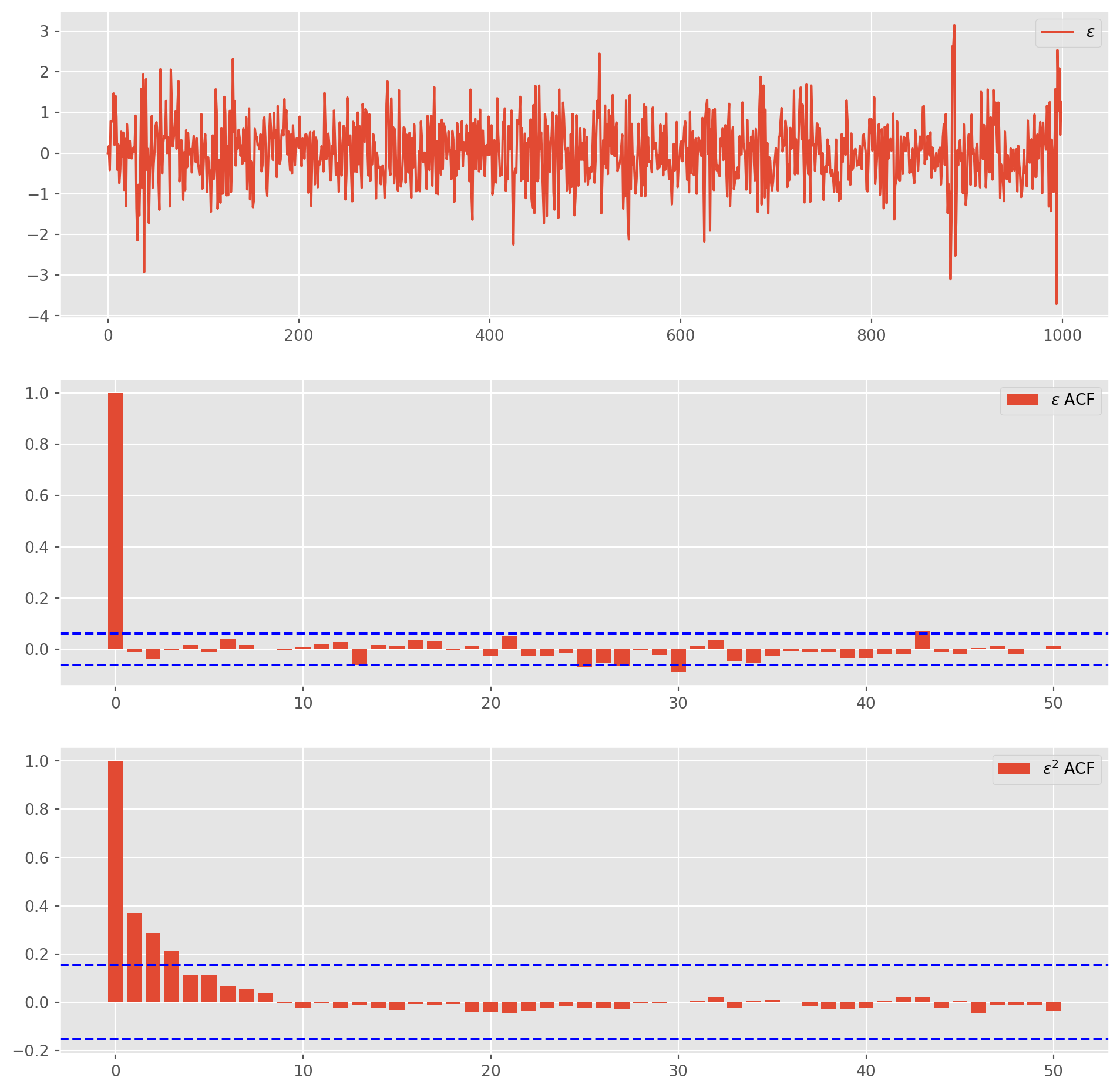
Note that \(\epsilon\) looks like white noise, in contrast \(\epsilon^2\) shows autocorrelation and volatility clustering.
model = arch.arch_model(epsilon, mean="Zero", vol="GARCH", p=1, o=0, q=1)
res = model.fit()
Iteration: 1, Func. Count: 5, Neg. LLF: 827535.1835085036
Iteration: 2, Func. Count: 10, Neg. LLF: 1151.346750915227
Iteration: 3, Func. Count: 15, Neg. LLF: 1150.5779430693185
Iteration: 4, Func. Count: 21, Neg. LLF: 1175.1702226992597
Iteration: 5, Func. Count: 26, Neg. LLF: 1112.519073761109
Iteration: 6, Func. Count: 30, Neg. LLF: 1112.5190355232094
Iteration: 7, Func. Count: 34, Neg. LLF: 1112.519033642905
Iteration: 8, Func. Count: 37, Neg. LLF: 1112.519033642824
Optimization terminated successfully (Exit mode 0)
Current function value: 1112.519033642905
Iterations: 8
Function evaluations: 37
Gradient evaluations: 8print(res.summary()) Zero Mean - GARCH Model Results
==============================================================================
Dep. Variable: y R-squared: 0.000
Mean Model: Zero Mean Adj. R-squared: 0.001
Vol Model: GARCH Log-Likelihood: -1112.52
Distribution: Normal AIC: 2231.04
Method: Maximum Likelihood BIC: 2245.76
No. Observations: 1000
Date: Sun, Oct 27 2024 Df Residuals: 1000
Time: 17:40:33 Df Model: 0
Volatility Model
==========================================================================
coef std err t P>|t| 95.0% Conf. Int.
--------------------------------------------------------------------------
omega 0.1455 4.705e-02 3.093 1.984e-03 [5.330e-02, 0.238]
alpha[1] 0.2516 5.495e-02 4.578 4.684e-06 [ 0.144, 0.359]
beta[1] 0.5074 0.112 4.520 6.191e-06 [ 0.287, 0.727]
==========================================================================
Covariance estimator: robustCompare estimated coefficients with our preset true value.
res.paramsomega 0.145524
alpha[1] 0.251595
beta[1] 0.507414
Name: params, dtype: float64Fitting Nasdaq Data
nasdaq = yf.download(
    ["^IXIC"],
    start=dt.datetime.today() - dt.timedelta(days=1500),
    end=dt.datetime.today(),
    progress=True,
    actions="inline",
    interval="1d",
)
[*********************100%***********************] 1 of 1 completednasdaq["log_ret"] = np.log(nasdaq["Adj Close"]) - np.log(nasdaq["Adj Close"].shift())
nasdaq = nasdaq.dropna()
nasdaq_acf = acf_func(nasdaq["log_ret"], nlags=50)fig, ax = plt.subplots(figsize=(12, 12), nrows=3, ncols=1)
ax[0].plot(nasdaq["Adj Close"], label="nasdaq 100")
ax[1].plot(nasdaq["log_ret"], label="Log Return")
ax[2].bar(np.arange(len(nasdaq_acf)), nasdaq_acf, label="nasdaq Return ACF")
ax[2].axhline(np.std(nasdaq_acf[1:]) * 1.96, ls="--", color="b")
ax[2].axhline(-np.std(nasdaq_acf[1:]) * 1.96, ls="--", color="b")
for i in range(3):
ax[i].legend()
plt.show()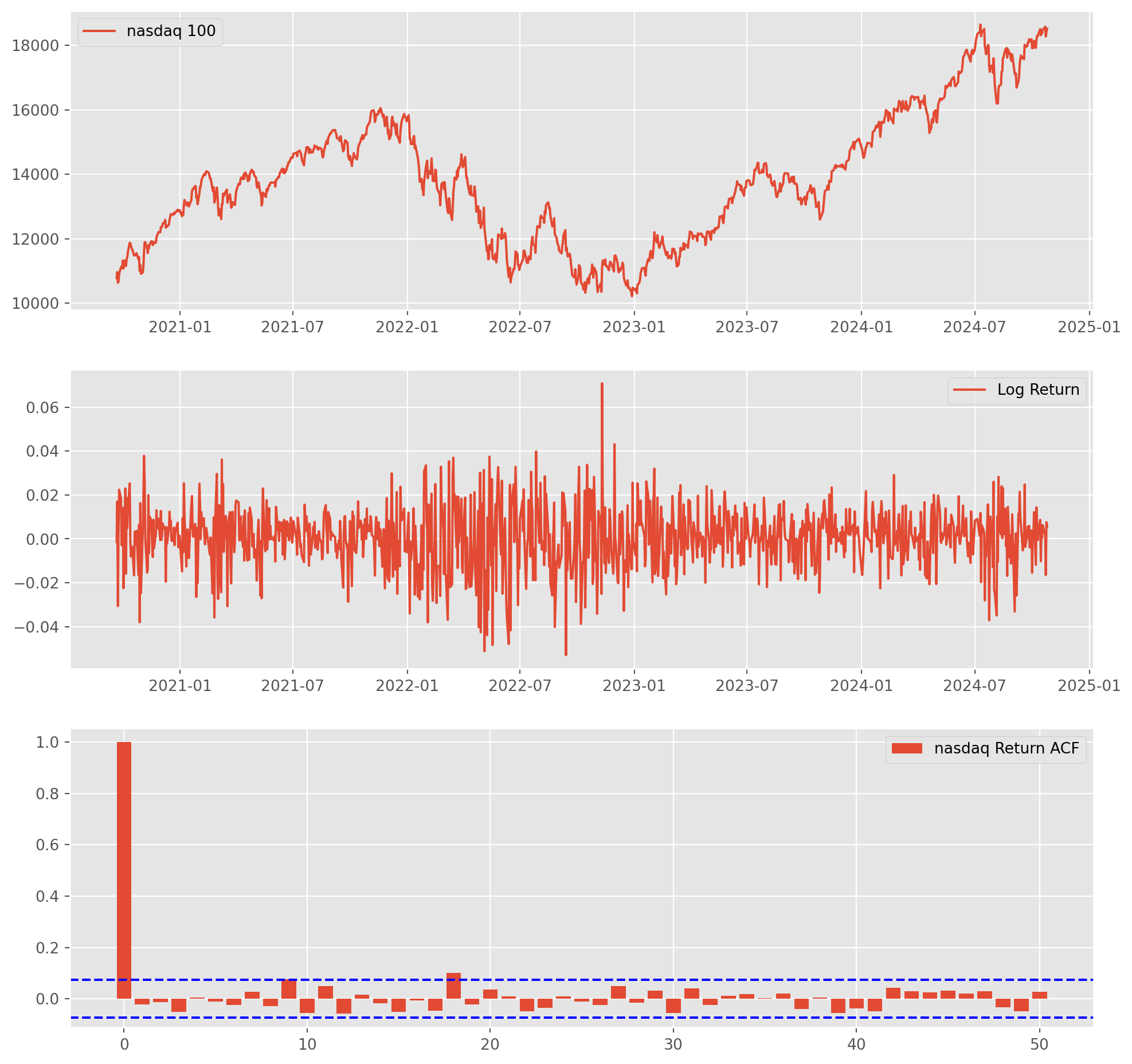
Fit the model with \(\text{ARIMA}\).
nasdaq.index = pd.DatetimeIndex(nasdaq.index).to_period(
    "D"
)  # without it, pandas will return warning
mod_obj = ARIMA(nasdaq["log_ret"], order=(2, 0, 2))
results = mod_obj.fit()Now we want to see how much can’t \(\text{ARIMA}\) explain away in residual.
resid_acf = acf_func(results.resid, nlags=50)
resid_sq_acf = acf_func(results.resid**2, nlags=50)
fig, ax = plt.subplots(figsize=(12, 8), nrows=2, ncols=1)
ax[0].bar(np.arange(len(resid_acf)), resid_acf, label="Residual ACF")
ax[0].axhline(np.std(resid_acf[1:]) * 1.96, ls="--", color="b")
ax[0].axhline(-np.std(resid_acf[1:]) * 1.96, ls="--", color="b")
ax[1].bar(np.arange(len(resid_sq_acf)), resid_sq_acf, label="Residual Squared ACF")
ax[1].axhline(np.std(resid_sq_acf[1:]) * 1.96, ls="--", color="b")
ax[1].axhline(-np.std(resid_sq_acf[1:]) * 1.96, ls="--", color="b")
for i in range(2):
ax[i].legend()
plt.show()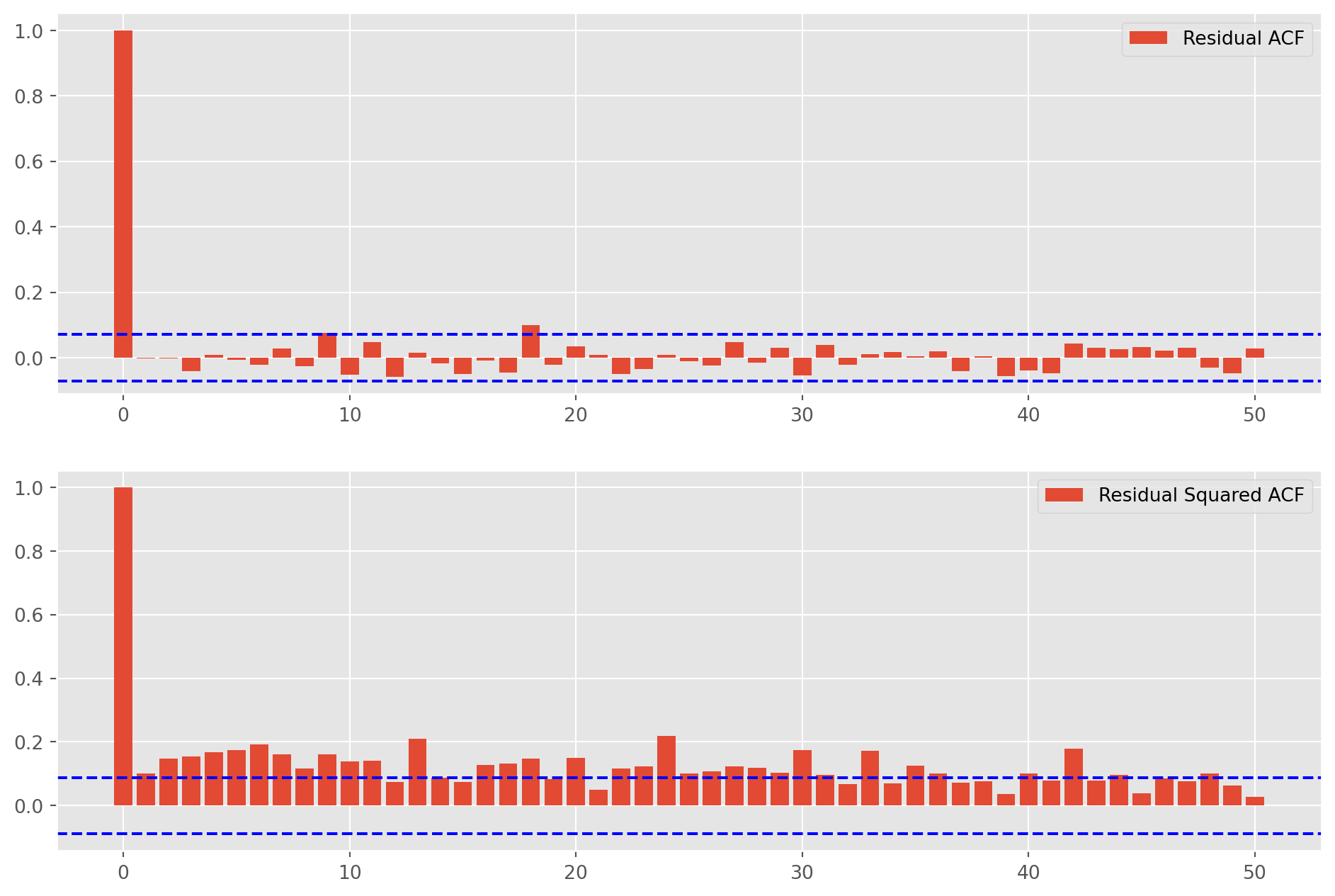
Auto correlation presents in the squared residuals, we are able to confirm conditional heteroskedastic behavior is present in the diff log return series of the Nasdaq.
Therefore, we can fit a \(\text{GARCH}\) model. Note, we are fitting the log return, not the residuals of \(\text{ARIMA}\).
model_garch = arch.arch_model(
    nasdaq["log_ret"], mean="Zero", vol="GARCH", p=1, o=0, q=1
)
res = model.fit()
Iteration: 1, Func. Count: 5, Neg. LLF: 827535.1835085036
Iteration: 2, Func. Count: 10, Neg. LLF: 1151.346750915227
Iteration: 3, Func. Count: 15, Neg. LLF: 1150.5779430693185
Iteration: 4, Func. Count: 21, Neg. LLF: 1175.1702226992597
Iteration: 5, Func. Count: 26, Neg. LLF: 1112.519073761109
Iteration: 6, Func. Count: 30, Neg. LLF: 1112.5190355232094
Iteration: 7, Func. Count: 34, Neg. LLF: 1112.519033642905
Iteration: 8, Func. Count: 37, Neg. LLF: 1112.519033642824
Optimization terminated successfully (Exit mode 0)
Current function value: 1112.519033642905
Iterations: 8
Function evaluations: 37
Gradient evaluations: 8resid_garch_sq = res.resid**2resid_garch_sq_acf = acf_func(resid_garch_sq, nlags=50)fig, ax = plt.subplots(figsize=(12, 4))
ax.bar(np.arange(len(resid_garch_sq_acf)), resid_garch_sq_acf)
ax.axhline(np.std(resid_garch_sq_acf[1:]) * 1.96, ls="--", color="b")
ax.axhline(-np.std(resid_garch_sq_acf[1:]) * 1.96, ls="--", color="b")
plt.show()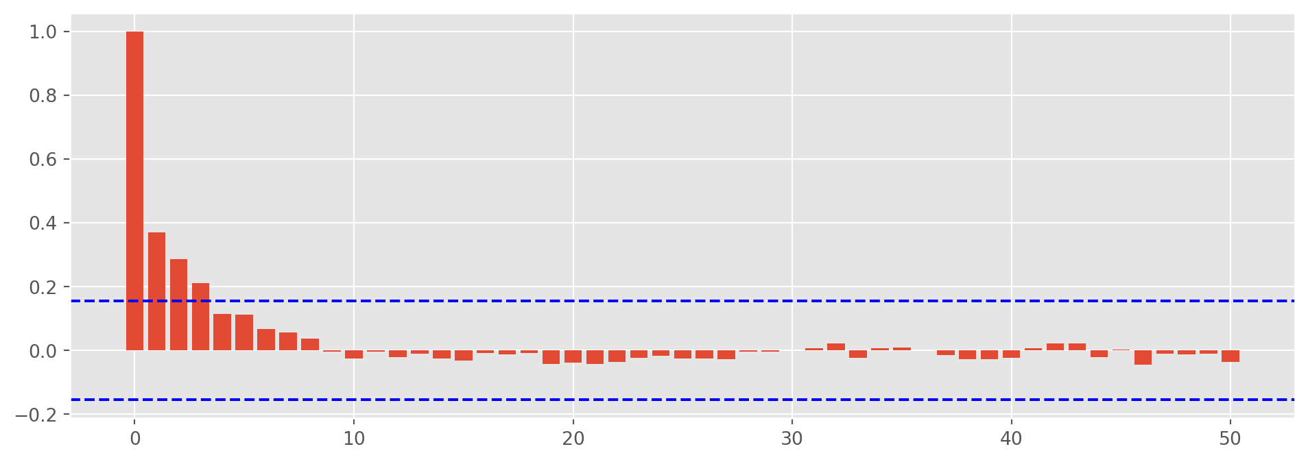
The residuals still shows autocorrelation, it could mean that model is misspecified, we will investigate further later.